Propensity Score
The propensity score makes it so that you don’t have to condition on the entirety of X to achieve independence of the potential outcomes on the treatment. It is sufficient to condition on this single variable, which is the propensity score
$$(Y_{0},Y_{1}) \perp T|e(x)$$
The propensity score is the conditional probability of receiving the treatment, right? So we can think of it as some sort of function that converts X into the treatment T. The propensity score makes this middle ground between the variable X and the treatment T. If we show this in a causal graph, this is what it would look like.
law of iterated expectations
$$E[X]=E[E[X|Y]]$$
Proof
具体内容参考统计学基础
其实我们可以看出,所谓$e(x)$就是$E[T|X]$也就是情形X下收到treatment的概率
$$E[T|e(x)]=E[E[T|e(x),X]|e(x)]=E[e(x)|e(x)]=e(x)$$
其中$E[T|e(x),X]=E[T|X]=e(x)$
Inverse Probability of Treatment Weighting (IPTW)
$$E[Y|X,T=1]-E[Y|X,T=0]=E\left[ \frac{Y}{e(x)}|X,T=1 \right]P(T)-E\left[ \frac{Y}{1-e(x)}|X,T=0 \right](1-P(T))$$直观上理解就是本来应该不被治疗的样本如果接受了治疗,那这个样本在分析的过程中会更加有价值
我们可以将其化简为$$E\left[ Y\frac{{T-e(x)}}{e(x)(1-e(x))} \right]$$
Proof
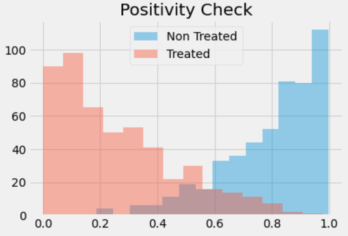
positivity assumption of causal inference: Notice that this estimator requires that $e(x)$ and $1−e(x)$ are larger than zero. In words, this means that everyone needs to have at least some chance of receiving the treatment and of not receiving it. Another way of stating this is that the treated and untreated distributions need to overlap.
Propensity Score Estimation
代码见11 - Propensity Score — Causal Inference for the Brave and True
Standard Error
首先考虑加权平均的方差$$\sigma^2_{w}=\frac{\sum_{i=1}^nw_{i}(y_{i}-\hat{\mu})^2}{\sum_{i=1}^nw_{i}}$$
However, we can only use this if we have the true propensity score. If we are using the estimated version of it, $\hat{P}(x)$, we need to account for the errors in this estimation process. The easiest way of doing this is by bootstrapping the whole procedure. This is achieved by sampling with replacement from the original data and computing the ATE like we did above. We then repeat this many times to get the distribution of the ATE estimate.
Common Issues with Propensity Score
Propensity score doesn’t need to predict the treatment very well. It just needs to include all the confounding variables.
To see this, consider the following example (adapted from Hernán’s Book). You have 2 schools, one of them apply the growth mindset seminar to 99% of its students and the other to 1%. Suppose that the schools have no impact on the treatment effect (except through the treatment), so it’s not necessary to control for it. If you add the school variable to the propensity score model, it’s going to have a very high predictive power. However, by chance, we could end up with a sample where everyone in school A got the treatment, leading to a propensity score of 1 for that school, which would lead to an infinite variance. This is an extreme example, but let’s see how it would work with simulated data.
其实就是当treatment和non treatment组之间特征没有过多的重叠时,对于接近0.5的概率附近样本较少,这会让方差增大This lack of balancing can generate some bias, because we will have to extrapolate the treatment effect to unknown regions.As a general rule of thumb, you are in trouble if any weight is higher than 20 (which happens with an untreated with propensity score of 0.95 or a treated with a propensity score of 0.05).
if the distributions don’t overlap, your data is probably not enough to make a causal conclusion anyway. To gain some further intuition about this, we can look at a technique that combines propensity score and matching
Propensity Score Matching
就是针对Propensity Score进行一次matching,从这个角度看,Propensity Score其实就是一种维度压缩,而我们就是再计算经过维度压缩后的特征的matching
值得注意的是,倾向性评分匹配并不适合bootstrap以估计SE[ON THE FAILURE OF THE BOOTSTRAP FOR MATCHING ESTIMATORS](On the Failure of the Bootstrap for Matching Estimators)
Thanks for watching! and this my learning note of the blog of Matheus Facure Alves.
感谢观看,这是我学习Matheus Facure Alves博客的笔记。
Cover image icon by Dewi Sari from Flaticon


