Beyond Confounders
Good Control
Sometimes treatment’s effect on the outcome is much smaller than other factors, in order to figure out the effect of treatment, we should control other factors because:
If a variable is a good predictor of the outcome, it will explain away a lot of its variance.
To demonstrate this, let’s resort to the partialling out way of breaking regression into 2 steps.
First, we will regress the treatment, email, and the outcome, payments, on the additional controls, credit limit and risk score.
Second, we will regress the residual of the treatment on the residuals of payments, both obtained in step 1. (This is purely pedagogical, in practice you won’t need to go through all the hassle).
To wrap it up, anytime we have a control that is a good predictor of the outcome, even if it is not a confounder, adding it to our model is a good idea. It helps lowering the variance of our treatment effect estimates. Here is a picture of what this situation looks like with causal graphs.
其实这里与我们之前将confounder针对treatment回归的有相似之处又有不同之处:
之前将confounder针对treatment的回归主要依赖于confounder同时对treatment和outcome有影响,所以我们需要打断confounder的路径,造成随机化的情况。
而这里的factor其实并非confounder,这里是由于多种因素同时存在造成的“大数吃小数”的情况,所以需要将factor对outcome回归后,在将残差对于treatment回归。
Bad Control
we should NOT add controls that are just good predictors of the treatment, because they will increase the variance of our estimates.
控制与treatment强相关的因素将会导致treatment的分组不均匀,从而提高variance,进而导致结果的不显著。
Selection Bias
selection bias is when we control for a common effect or a variable in between the path from cause to effect.(参考[[Graph Casual Model]]中的Selection Bias)
Here is some examples:
- Adding a dummy for paying the entire debt when trying to estimate the effect of a collections strategy on payments.
- Controlling for white vs blue collar jobs when trying to estimate the effect of schooling on earnings
- Controlling for conversion when estimating the impact of interest rates on loan duration
- Controlling for marital happiness when estimating the impact of children on extramarital affairs
- Breaking up payments modeling E[Payments] into one binary model that predict if payment will happen and another model that predict how much payment will happen given that some will: E[Payments|Payments>0]*P(Payments>0)
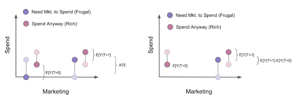
COP: A special case of Selection Bias
这个问题来自与一个常见的问题:如果遇到0,是否要将其舍去,其实这个问题就是针对舍去0的模型:
我们在针对一些相对稀疏的outcome进行推断时,常常倾向于删去0值,但是这样会导致我们舍去了一部分正常为0的数据,以基因表达为例;
如果我们对于某群体给予某种药物,则必然有一部分基因在大部分情况下均不表达,这时有人提出:为什么我们不只看那部分表达的个体在治疗前后的基因表达改变的情况。
但是,这个想法是错误的!
直观上讲,就是我们大可以将群体分为2群,一群是在药物治疗后基因表达增加,而这个群体本身就有基因表达;二群是在药物治疗后基因表达从0到1,这个群体本身无基因表达。如果我们简单去掉0数据,则可能带来:二群的治疗前的数据的丢失。最后在研究因果效应时会导致因果效应偏小。
理论上推导如下:
上式子中,前者代表“Participation Effect”,及治疗前后值从0到1的改变情情况,即一群的预期效益;后者则代表”COP”,即治疗前后增加的基因表达数量,即二群的预期效益
数学上完全正确,问题出在估计$E[Y|Y>0|T=1]-E[Y|Y>0|T=0]$过程中
这就是我们常见的bias公式,我们可以看到,前面的那个估计正确,但是后面可能会出现bias,也就是说$E[Y_{0}|Y_{1}>0]<E[Y_{0}|Y_{0}>0]$, 因为会有部分$Y_{0}=0$的情况被排除。
注意:上式子我们需要求得的是$E[Y_{1}-Y_{0}|Y_{1}>0]$,其中$E[Y|T=1]-E[Y|T=0]$,是我们观察到的数据,主要问题就是我们在计算过程中可能会把$E[Y_{0}|Y_{1}>0]-E[Y_{0}|Y_{0}>0]$所忽视
这里的思路类似于[[mathematic/Casual inference/Introduction]]中的思路,就是计算ATT,但是我们加了个前提就是要大于0,大于0就让无法ATT的转化无法正常进行,因为这使得引入了新的bias,很奇妙吧,虽然过程不同,但是最后归于公式的时候却是相同的
相当有趣的是这里我们依旧可以用Selection Bias解释,这是因为治疗与否影响了基因表达是否大于0,同时outcome也对基因表达是否大于0有影响,构成了一个Collider,一旦控制,就会带来Selection Bias.
Thanks for watching! and this my learning note of the blog of Matheus Facure Alves.
感谢观看,这是我学习Matheus Facure Alves博客的笔记。
Cover image icon by Dewi Sari from Flaticon


